

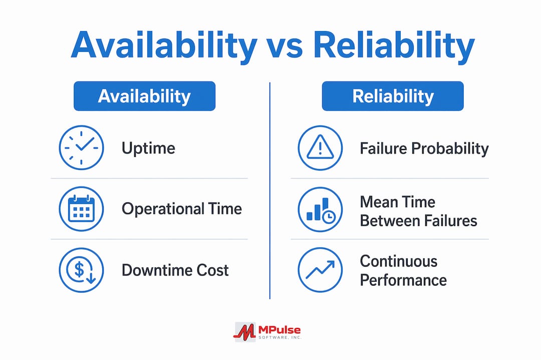
Availability measures the fraction of time a system is operational; reliability measures the probability it performs without failure over a specified interval. The two are related but distinct signals. Availability is calculated as MTBF / (MTBF + MTTR), expressed as a percentage over a measurement window. Reliability, for repairable systems, is typically expressed using MTBF-based models; for non-repairable components, MTTF applies. Under a constant failure rate assumption, reliability over an interval t equals exp(−λt), where λ = 1/MTBF. A system with an MTBF of 1,000 hours and an MTTR of 1 hour yields availability of 1,000 / (1,000 + 1) = 99.9%, which corresponds to roughly 8 hours 45 minutes of allowed downtime per year. Two systems can both report 99.9% uptime while delivering completely different user experiences: one with 500 two-minute outages spread across the year, another with a single 8-hour event. The uptime percentage is identical; the operational impact is not.
Table of Contents
- What does availability actually measure?
- What does reliability mean, and how do you measure it?
- How do availability and reliability relate to each other?
- Key metrics and formulas every operations team should track
- How to improve availability through engineering and operational controls
- How to improve reliability by reducing failure frequency
- How maintainability reduces MTTR and improves uptime
- Common failure types, detection signals, and how to respond
- Operationalizing reliability: what the research says goes beyond uptime
- What your team should monitor, alert on, and review regularly
- Key Takeaways
- The metrics that matter most are the ones tied to business impact
- MPulse CMMS helps you turn reliability data into action
- Useful sources for further reading
- FAQ
What does availability actually measure?
Availability is the proportion of time a system can perform its intended function, measured at a given instant or over a defined window. The two most common formulas are:
- Uptime percentage: (Elapsed time − Downtime) / Elapsed time × 100
- MTBF-based: MTBF / (MTBF + MTTR)
Both express the same concept: how much of the clock does the system spend in a usable state?
The “nines” shorthand and what they cost you
The table below converts availability percentages into concrete downtime allowances. These figures assume a calendar year of 8,760 hours.
| Availability | Annual downtime | Weekly downtime |
|---|---|---|
| 99% (two nines) | ~87 hours 36 min | ~1 hour 41 min |
| 99.9% (three nines) | ~8 hours 45 min | ~10 min 5 sec |
| 99.99% (four nines) | ~52 minutes 34 sec | ~1 min 0 sec |
| 99.999% (five nines) | ~5 minutes 15 sec | ~6 sec |
Each step up the table is not a linear improvement. Moving from three nines to four typically requires multi-region deployments, automated failover, and sophisticated health checks. The fifth nine demands techniques that most teams find disproportionately expensive relative to the business benefit.
Measurement windows and SLA implications
Measurement windows matter as much as the formula. A rolling 30-day window penalizes recent incidents more heavily than a calendar-year window does, which is why SLAs often specify the window explicitly. Planned maintenance is another variable: some SLAs exclude scheduled downtime from the denominator, which can inflate reported availability significantly. Teams should confirm whether their SLA counts planned maintenance windows as downtime before signing.
Common pitfalls when interpreting availability numbers:
- Partial degradation counted as “up”: A system that responds to health checks but serves errors to users is technically “available” by most monitors.
- Monitoring blind spots: If your probe runs every 60 seconds, a 45-second outage is invisible to the metric.
- Aggregated availability masking regional failures: A global average can hide a region that is completely down.
What does reliability mean, and how do you measure it?
Reliability is the probability a system performs its intended function without failure over a specified time interval, under stated conditions. Where availability asks “is the system up right now?”, reliability asks “will it stay up for the next 500 hours?”
MTBF vs. MTTF: choosing the right model
MTBF (Mean Time Between Failures) applies to repairable systems. It is the average elapsed time between the end of one failure and the start of the next. MTTF (Mean Time to Failure) applies to non-repairable components, measuring the expected time until the first and only failure.
Under the constant failure rate assumption, the reliability function is:
R(t) = e^(−λt) where λ = 1/MTBF
Worked example: A pump has an MTBF of 2,000 hours. What is the probability it runs without failure for 500 hours?
- λ = 1/2,000 = 0.0005 failures/hour
- R(500) = e^(−0.0005 × 500) = e^(−0.25) ≈ 0.779
There is roughly a 78% probability the pump completes 500 hours without a failure. That figure drops to about 61% at 1,000 hours and 37% at 2,000 hours, illustrating how reliability degrades over time even when MTBF is constant.
What to record and common measurement pitfalls
Accurate reliability measurement requires logging every failure event with a timestamp, distinguishing hard failures (full loss of function) from service degradation (partial loss). Clustered failures — multiple failures triggered by a single root cause — should be recorded as one event for MTBF purposes, not counted separately. Correlated failures across redundant components are a particularly dangerous blind spot: two “independent” servers that share a power circuit are not statistically independent.
How do availability and reliability relate to each other?
The formula MTBF / (MTBF + MTTR) makes the relationship explicit. Availability depends on both how often failures occur (MTBF, a reliability signal) and how quickly they are resolved (MTTR, a maintainability signal). Improving either one raises availability, but through entirely different mechanisms.
This coupling creates divergence scenarios that matter operationally:
- High availability, low reliability: MTTR is very short, so even frequent failures barely dent the uptime percentage. A system that fails 20 times a day but recovers in 30 seconds each time can still report 99.9% availability. Users experience constant disruption; the metric looks fine.
- High reliability, lower availability: Failures are rare (high MTBF), but when one occurs, repair takes hours. A manufacturing line that runs flawlessly for months but requires a 12-hour repair when it does fail may post lower availability than a system that fails more often but recovers in minutes.
- Both high: The target state — rare failures and fast recovery. Achieved through preventive maintenance, redundancy, and well-practiced incident response.
- Both low: The crisis state — frequent failures and slow recovery. Usually signals systemic design or process problems.
When to prioritize which metric
Availability is the right primary signal for customer-facing, always-on services where any downtime directly affects revenue or user experience. Reliability is the more important signal for safety-critical or correctness-critical systems, where a failure during operation carries consequences beyond lost uptime. A medical device, a flight control system, or a financial settlement process needs high reliability; a marketing website needs high availability. Most enterprise systems need both, but the trade-off decisions differ by context.
High availability percentages can mask degraded performance; a system that responds to health checks while serving slow or partial results is technically “up” but operationally unreliable. That gap is where user-centric SLOs become more informative than raw uptime numbers.
Key metrics and formulas every operations team should track
MTBF and MTTR are the two foundational inputs for availability calculations. The table below defines each metric, its formula, and where to source the data.
| Metric | Formula | Data source | Used for |
|---|---|---|---|
| MTBF | Total uptime / Number of failures | Incident logs | Reliability baseline, availability input |
| MTTF | Total operating time / Number of units failed | Asset lifecycle records | Non-repairable component planning |
| MTTR | Total repair time / Number of repairs | Work order logs | Availability input, maintainability signal |
| Availability % | MTBF / (MTBF + MTTR) × 100 | Monitoring + incident logs | SLA compliance, uptime reporting |
| Error budget | (1 − SLO) × measurement window | SLO definition | Release velocity vs. stability trade-off |
| SLO | Target availability or latency threshold | Business/product decision | Internal reliability target |
| SLA | Contractual availability commitment | Customer contract | External accountability |
Worked calculations
Availability from MTBF and MTTR:
A server with an MTBF of 500 hours and an MTTR of 2 hours would have an availability of about 99.6% (calculated as 500 / (500 + 2) × 100 ≈ 99.6%).
Error budget consumption:
Your SLO is 99.9% over 30 days (43,200 minutes). Your error budget is 0.1% × 43,200 = 43.2 minutes. After three incidents totaling 30 minutes of downtime, you have 13.2 minutes of budget remaining. A fourth incident of 15 minutes would exhaust the budget and trigger a freeze on non-critical deployments.
At five or six nines of availability, monitoring measurement error can exceed the actual downtime you are trying to measure. Design your measurement system before optimizing for tiny downtimes — multiple observers and cross-checks are not optional at that level.
How to improve availability through engineering and operational controls
Availability improvements fall into two categories: reducing the frequency of failures (a reliability problem) and reducing the time to recover when failures occur (a maintainability problem). The controls below address both.
Redundancy and failover:
Active/passive redundancy keeps a standby component ready to take over when the primary fails. Active/active configurations distribute load across multiple instances, so a single failure reduces capacity rather than causing an outage. Automatic failover removes the human delay from recovery, which directly compresses MTTR.

Deployment strategies:
Blue/green deployments maintain two identical production environments, allowing instant rollback if a release introduces failures. Canary deployments route a small percentage of traffic to the new version first, limiting blast radius if something goes wrong. Both strategies reduce the availability impact of software changes.
Graceful degradation and feature flags:
A system that can shed non-critical features under load or during partial failures maintains core functionality rather than failing completely. Feature flags let teams disable specific capabilities without a full deployment, reducing the time to mitigate an incident.
Operational controls:
Maintenance windows should be scheduled during low-traffic periods and communicated clearly in runbooks. Rolling upgrades apply changes to one node at a time, keeping the rest of the system operational. Runbooks and operational playbooks document the exact steps for common failure scenarios, so on-call engineers spend time executing rather than diagnosing.
Pro Tip: When pursuing four or five nines, measure your monitoring system’s own accuracy first. If your uptime probe has a 60-second polling interval and your alerting pipeline adds another 30 seconds of latency, you cannot reliably detect or attribute sub-90-second outages — and those outages still count against your SLA.
Preventive maintenance scheduling through a CMMS reduces unplanned downtime by catching asset degradation before it becomes a failure. MPulse Software’s IIoT monitoring integrations feed real-time sensor data into maintenance workflows, allowing teams to act on condition-based alerts rather than waiting for a failure event.
How to improve reliability by reducing failure frequency
Reliability improvements target MTBF directly: fewer failures over the same operating period. The steps below are sequenced from foundational to advanced.
- Establish a preventive maintenance program. Schedule inspections, lubrication, calibration, and component replacements based on manufacturer intervals or historical failure data. A CMMS-driven maintenance schedule automates these triggers and tracks completion, removing the human error of missed service intervals.
- Implement condition-based maintenance. Sensor data (vibration, temperature, pressure) can detect degradation before failure. Condition-based triggers replace fixed-interval schedules with evidence-based ones, extending MTBF without over-maintaining assets.
- Conduct root-cause analysis after every significant failure. A structured RCA process (5-Why, fishbone, fault tree) identifies the systemic cause rather than the proximate one. Without this step, teams fix symptoms and the same failure recurs.
- Apply automated testing and chaos engineering. For software systems, automated regression tests catch regressions before they reach production. Chaos engineering deliberately injects failures in controlled conditions to expose hidden dependencies and single points of failure.
- Isolate dependencies and reduce blast radius. Circuit breakers, bulkheads, and timeout policies prevent a failure in one component from cascading to others. Microservice architectures that share databases or message queues are particularly vulnerable to this pattern.
- Track component lifecycle and enforce change control. Components approaching end-of-life should trigger planned replacements, not reactive ones. Change control processes ensure that modifications to production systems are reviewed, tested, and reversible.
- Review error budgets at a regular cadence. When the error budget is nearly exhausted, reliability work takes priority over new feature delivery. This is a policy decision, not a technical one, and it needs explicit organizational buy-in.
Pro Tip: Prioritize reliability investments by business impact, not failure frequency. A component that fails rarely but causes a four-hour outage when it does deserves more investment than one that fails often but recovers in seconds. Map failure modes to revenue or safety impact before allocating engineering effort.
How maintainability reduces MTTR and improves uptime
Maintainability is the ease and speed with which a system can be restored to full operation after a failure. It directly controls MTTR, which in turn controls availability. A system with excellent reliability but poor maintainability can still post disappointing availability numbers when failures do occur.
Practical maintainability improvements include:
- Spare parts strategy: Critical components with long lead times should be stocked on-site. A 48-hour wait for a replacement part is 48 hours of MTTR that could be eliminated.
- Modular design: Systems designed for component-level replacement rather than full-unit replacement reduce repair time significantly. A modular power supply that swaps in 10 minutes beats a monolithic unit requiring a 4-hour rebuild.
- Remote diagnostics: Monitoring dashboards and remote access tools allow engineers to diagnose failures before physically arriving at the asset, compressing the time-to-diagnosis portion of MTTR.
- Documentation and runbooks: Accurate, current documentation means the on-call engineer does not spend the first 30 minutes of an incident figuring out the system architecture. Runbooks should cover the most common failure modes with step-by-step resolution procedures.
- On-call playbooks: Escalation paths, contact lists, and decision trees for ambiguous situations reduce coordination overhead during incidents.
- Personnel qualification tracking: An engineer who is not qualified to work on a specific asset type cannot begin the repair until a qualified technician arrives. MPulse Software’s personnel qualification tracking features ensure the right person is dispatched to the right job, removing a common source of MTTR inflation.
Work order management is the operational link between a failure event and its resolution. Connecting incident detection to corrective work orders automatically creates a documented repair record, tracks time-to-resolution, and feeds MTTR calculations without manual data entry.

Common failure types, detection signals, and how to respond
Failures cluster into recognizable categories. Knowing the category early narrows the response path.
- Hardware failures: Physical component degradation or sudden failure. Detection signals: hardware health alerts, SMART data for drives, temperature sensors, vibration anomalies. Response: isolate the affected component, activate spare or redundant path, initiate replacement work order.
- Software failures: Bugs, memory leaks, deadlocks, or configuration errors in application code. Detection signals: error rate spikes, latency increases, process crashes, log anomalies. Response: roll back the recent deployment or restart the affected service; capture a heap dump or log snapshot before restarting.
- Network failures: Packet loss, routing failures, DNS resolution errors, or bandwidth saturation. Detection signals: synthetic checks failing from external probes, latency spikes, connection timeout errors. Response: verify physical connectivity, check routing tables, confirm DNS resolution, engage ISP or network team.
- Configuration failures: Incorrect settings applied during a change window. Detection signals: failures that correlate precisely with a recent change event. Response: revert the configuration change; do not attempt to fix forward until the system is stable.
- Cascading failures: A failure in one component triggers failures in dependent components. Detection signals: multiple services failing simultaneously, error rates rising across unrelated systems. Response: identify and isolate the origin component; shed load from downstream services using circuit breakers or feature flags.
- Environmental failures: Power, cooling, or physical environment issues. Detection signals: UPS alerts, temperature alarms, facility monitoring. Response: activate backup power or cooling; initiate controlled shutdown if environment cannot be stabilized.
For each failure type, the response sequence follows the same pattern: detect → isolate → mitigate → restore → post-incident review. The post-incident review is not optional. Without it, the failure recurs.
Integrating failure detection with CMMS work order flows closes the loop: an alert triggers a work order, the work order documents the repair, and the repair data feeds MTBF and MTTR calculations for the next planning cycle.
Operationalizing reliability: what the research says goes beyond uptime
Uptime percentage is a necessary metric, but it is not sufficient for operational reliability. The IEEE/IEC dependability framework formalizes this by treating availability and reliability as two components of a larger structure that also includes maintainability and safety. Teams that optimize only for uptime percentage often find themselves with systems that are technically “available” but operationally fragile.
Practitioner research points to three areas where teams consistently underinvest:
Error budgets and SLO design. An error budget translates an abstract SLO into a concrete operational policy. When the budget is healthy, teams can deploy freely. When it is nearly exhausted, reliability work takes priority. This creates a self-correcting feedback loop that uptime dashboards alone cannot provide. Practitioners should translate reliability goals into customer-impact SLOs rather than chasing abstract uptime numbers.
Observability over monitoring. Traditional monitoring checks whether a system is up. Observability asks why it behaved the way it did. Structured logging, distributed tracing, and metric correlation allow teams to diagnose novel failure modes without pre-defining every possible alert condition.
Resilience engineering in distributed systems. Microservice architectures introduce failure modes that monolithic systems do not have: network partitions, partial availability, and cascading timeouts. Chaos engineering practices deliberately expose these failure modes in controlled conditions before they surface in production.
What your team should monitor, alert on, and review regularly
Monitoring checklist
- Four golden signals: Latency (how long requests take), traffic (demand volume), errors (rate of failed requests), and saturation (how close resources are to capacity). Combining these signals with synthetic checks gives a complete picture of system health.
- Synthetic checks: Scripted transactions that simulate real user actions against critical paths. These catch failures that internal health checks miss.
- Business-key transactions: Instrument the specific workflows that generate revenue or fulfill compliance requirements. A payment processing flow or a regulatory reporting job deserves its own SLO.
- SLO burn rate alerts: Alert when the error budget is being consumed faster than the SLO allows, not just when it is exhausted. A burn rate alert gives teams time to act before the budget runs out.
Questions to ask during reliability reviews
- What is our current MTBF for each critical asset or service, and is it trending up or down?
- How is MTTR trending over the past 90 days? Are we getting faster or slower at recovery?
- Where are the single points of failure in this system, and what is the plan if each one fails?
- Which failure modes from the last quarter have not yet had a root-cause fix implemented?
- Is our error budget on track for the current measurement window?
CMMS-linked checklist items
- Are preventive maintenance work orders completing on schedule, or are they being deferred?
- Are spare parts for critical components stocked at the required levels?
- Are personnel qualifications current for all assets in the critical path?
- Are failure events from the field being captured in the CMMS and feeding MTBF calculations?
Key Takeaways
Availability and reliability are related but operationally distinct signals: availability measures the fraction of time a system is operational, while reliability measures the probability it performs without failure over a specified interval, and improving both requires targeting MTBF, MTTR, and maintainability together.
| Point | Details |
|---|---|
| Availability formula | Calculate as MTBF / (MTBF + MTTR); 99.9% permits roughly several hours of downtime per year. |
| Reliability formula | Use R(t) = e^(−λt) with λ = 1/MTBF; a system with MTBF of 2,000 hours has ~78% reliability over 500 hours. |
| Metrics to track | MTBF, MTTR, MTTF, error budget, and SLOs together give a complete picture that uptime % alone cannot. |
| Improving both signals | Redundancy and failover reduce MTTR; preventive and condition-based maintenance increase MTBF. |
| MPulse Software | MPulse CMMS automates preventive maintenance schedules, tracks work orders, and integrates IIoT monitoring to reduce unplanned downtime and improve MTBF and MTTR data accuracy. |
The metrics that matter most are the ones tied to business impact
Most operations teams I work with start in the same place: a dashboard showing uptime percentage, and a vague sense that the number should be higher. The problem is that uptime percentage answers the wrong question. It tells you how often the system was technically available; it does not tell you whether users could actually accomplish what they came to do.
The more useful framing is to ask: which failures actually affected users, and how long did it take to restore full function? That question leads you to user-centric SLOs, error budgets, and MTTR tracking — metrics that connect directly to business outcomes rather than infrastructure states.
The trade-off between availability and reliability is also more nuanced than most guides acknowledge. Chasing an additional “nine” of availability often requires architectural changes that introduce new failure modes. A multi-region active/active deployment eliminates single-region outages but creates split-brain scenarios, replication lag, and cross-region latency that a single-region system never had to handle. The engineering effort is real, and so is the new risk surface. Teams should make that trade explicitly, with a clear-eyed view of what they are gaining and what they are adding.
Preventive maintenance is undervalued in software-centric organizations and overdue for attention in asset-heavy ones. The data is consistent: systems that receive scheduled, documented maintenance have higher MTBF and lower MTTR than systems maintained reactively. That is not a surprising finding, but the gap between knowing it and operationalizing it is where most teams struggle. A CMMS that automates scheduling, tracks completion, and feeds failure data back into planning closes that gap systematically.
MPulse CMMS helps you turn reliability data into action
Knowing your MTBF and MTTR numbers is only half the work. The other half is building the operational workflows that move those numbers in the right direction. MPulse Software connects preventive maintenance automation, real-time IIoT monitoring, and work order management into a single platform, so the data from your monitoring systems flows directly into the maintenance actions that improve reliability.

Preventive maintenance schedules run automatically based on calendar intervals or condition-based triggers from connected sensors. Work orders capture repair time and failure data, feeding the MTBF and MTTR calculations your team needs for SLO planning. Personnel qualification tracking confirms that the right technician handles each asset, removing a common source of MTTR delay. Over 3,500 customers rely on MPulse CMMS to reduce unplanned downtime and build the maintenance records that support compliance and audit requirements.
See how MPulse CMMS maps to your reliability program: explore the full platform or review the IIoT and real-time monitoring capabilities that feed condition-based maintenance workflows.
Useful sources for further reading
- IEEE Technology Navigator: Dependability — The authoritative reference for the IEC/IEEE dependability framework, covering reliability, availability, maintainability, and safety as a unified structure.
- Addy Osmani: Service Reliability Mathematics — Practitioner-focused treatment of reliability math, the “nines” table, error budgets, and the measurement accuracy problem at high availability levels.
- Sedai: Service Reliability Definition, Metrics & Best Practices — Covers the four golden signals, observability practices, and why uptime alone does not capture user-perceived reliability.
- Atlassian: Reliability vs. Availability — Clear comparison of the two metrics with formula definitions and incident management context.
- IBM: MTTR vs. MTBF — Practical definitions and operational guidance for MTBF and MTTR, including how each feeds availability calculations.
FAQ
What is the difference between availability and reliability?
Availability measures the fraction of time a system is operational, expressed as a percentage. Reliability measures the probability a system performs without failure over a specified interval, typically expressed using MTBF or MTTF-based models.
What is MTBF and MTTR, and how do they relate to availability?
MTBF (Mean Time Between Failures) is the average time between the end of one failure and the start of the next; MTTR (Mean Time To Repair) is the average time to restore the system after a failure. Availability is calculated directly from both: MTBF / (MTBF + MTTR).
What are the four elements of reliability in a dependability framework?
The IEEE/IEC dependability framework defines four core attributes: reliability (continuity of correct service), availability (readiness for correct service), maintainability (ability to be repaired), and safety (absence of catastrophic consequences). Reliability and availability are the two attributes directly measurable through quantitative metrics.
What are the three types of availability?
Availability is commonly categorized as inherent availability (based on MTBF and MTTR under ideal conditions), achieved availability (accounting for preventive maintenance time), and operational availability (reflecting all scheduled and unscheduled downtime in real operating conditions). Operational availability is the most conservative and most realistic figure for planning purposes.
How do error budgets connect SLOs to reliability decisions?
An error budget is the allowed downtime or failure rate derived from an SLO: a 99.9% SLO over 30 days yields 43.2 minutes of error budget. When that budget is nearly consumed, teams pause non-critical deployments and prioritize reliability fixes, creating a direct link between reliability metrics and engineering decisions.